gws_plate_reader

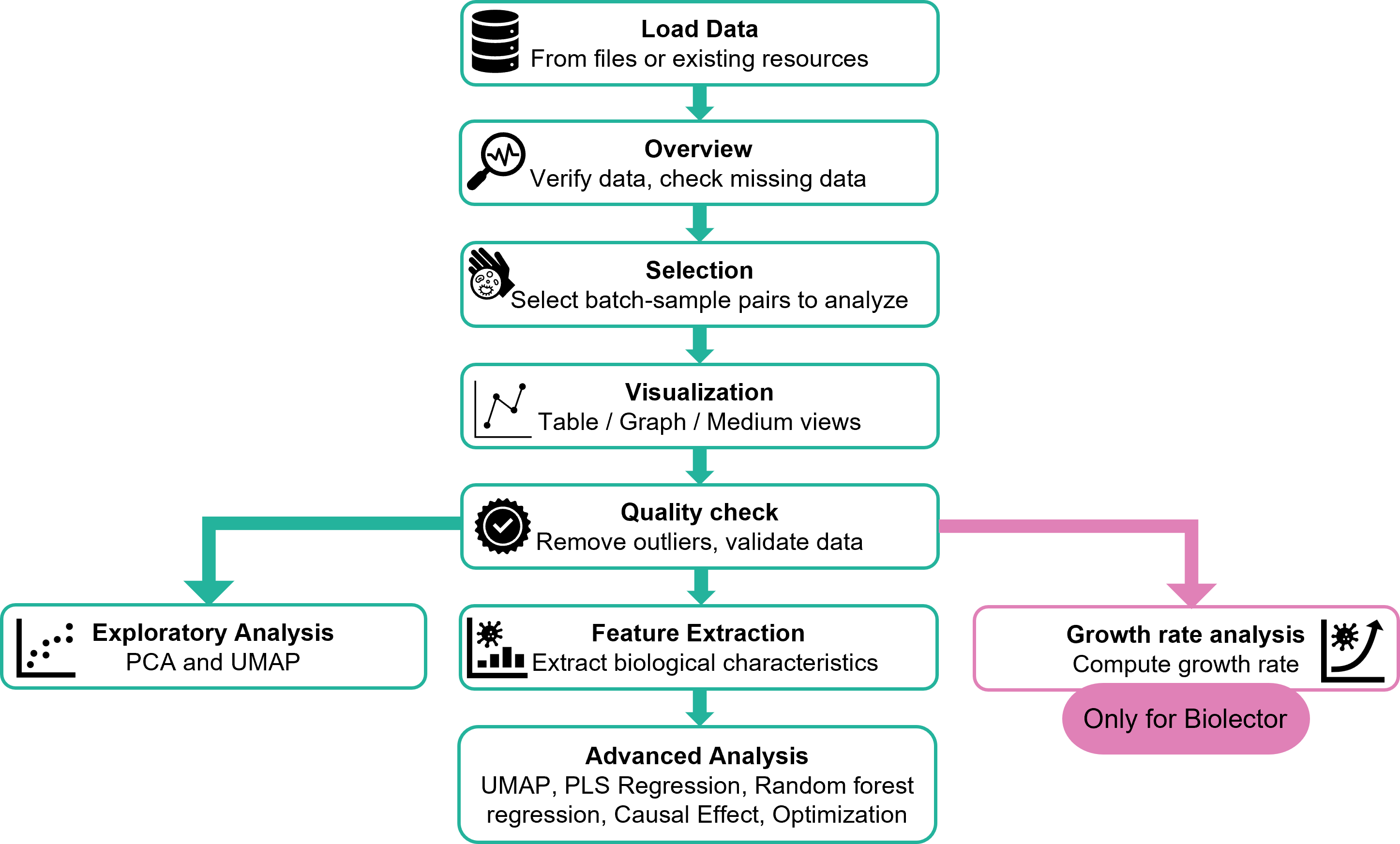
Constellab Bioprocess is a data analysis application designed to streamline the processing, visualization, and analysis of bioprocess data generated from Biolector systems and fermentors.

The application centralizes all fermentation-related data in a single platform and provides users with ready-to-use, standardized analysis pipelines. Through an intuitive dashboard interface, users can run analyses and visualize results using simple button-driven workflows — without needing to write code.

The main goal of Constellab Bioprocess is to accelerate data interpretation, improve consistency of analysis, and ensure traceability across bioprocess experiments.

▶

Click here if you want to follow a use case: https://constellab.community/stories/2e1022d3-1494-44e8-a801-5de029b2ff83/find-the-optimal-medium-with-constellab-bioprocess-use-case

Where to begin?

First, add the 'gws_design_of_experiment' and 'gws_plate_reader' bricks to your lab.

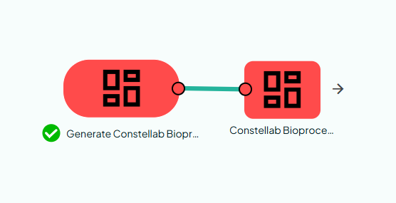
Next, create a new scenario and add the 'Generate Constellab Bioprocess Dashboard app' task. Click on 'Add an output' and run the scenario.

You can then open the app by clicking on the output.

Start by creating a new recipe. Then, choose whether it will be a Fermentor or Biolector recipe.

Next, give your recipe a clear, descriptive name and select your data. You can upload files from your computer or import them directly from Constellab.

🧪 Fermentor Recipe

The fermentor recipe is handled by ConstellabBioprocessLoadData and requires 4 files:

1. Info CSV — Required

A CSV file containing experiment and fermenter information.

Each row maps a fermentor to its batch and medium.

2. Raw Data CSV — Required

A CSV file containing the time-series measurement data from the fermentors (e.g., OD, pH, dissolved oxygen, temperature, etc.).

3. Medium CSV  — Required

A CSV file describing the composition of each medium referenced in the Info CSV.

4. Follow-up ZIP — Required

A ZIP archive containing follow-up/offline measurement files (e.g., manual sampling data, offline OD measurements, metabolite concentrations).

🧫 BiolectorXT (Microplate) Recipe

The BiolectorXT recipe is handled by BiolectorXTLoadData and supports multiple plates. For each plate, you provide a set of files, plus one shared medium table across all plates.

Shared across all plates

• Medium Composition Table — Optional

A CSV/Table describing the composition of each medium used across all plates.

Per plate

Raw data — Required

A Table containing the raw BiolectorXT measurement data with the following columns:

Folder Metadata — Required

A ZIP/Folder containing the BiolectorXT JSON metadata file(s). The folder must contain a file ending with BXT.json. This file includes:

• Channels: List of measurement channels/filters
• Microplate: Well configurationCultivationLabels: Wells used for cultivation (e.g., ["A01", "A02", ...])ReservoirLabels: Wells used as reservoirs (e.g., ["C01", "C02", ...])
• CultivationLabels: Wells used for cultivation (e.g., ["A01", "A02", ...])
• ReservoirLabels: Wells used as reservoirs (e.g., ["C01", "C02", ...])
• Layout: Well label descriptions

Info Table — Optional

A CSV/Table mapping wells to their medium names and additional metadata.

🔎 Biolector/Fermentor Comparison Recipe

  The Biolector/Fermentor Comparison recipe allows you to compare the performance of Biolector and fermentor experiments for the same process. It generates overlay plots and computes summary statistics to facilitate comparison between the two cultivation systems.  

Select : 

• one Biolector recipe and one QC step
• one Fermentor recipe and one QC step

Once everything is set, click Create recipe.

You will then see a table summarizing all your recipes. This table is useful for retrieving, reviewing, and comparing your previous analyses over time.

Click on the recipe you want to view.

You will be redirected to the recipe details page, where you will first see an overview of your dataset.

Overview

The starting point of your analysis. This step displays the results of the data loading scenario and helps you verify data quality.

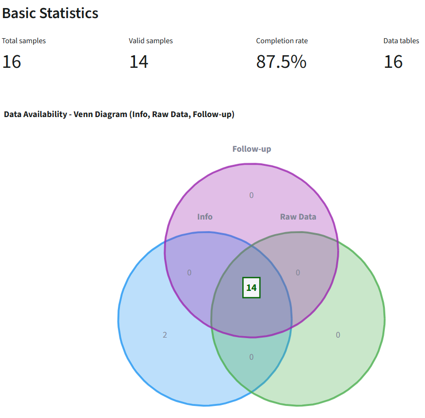
What you'll see:

• Basic Statistics (4 key metrics):
• Total Samples: Total number of batch-sample pairs found in info file
• Valid Samples: Number of complete samples (all data types present)
• Completion Rate: Percentage of samples with complete data
• Data Tables: Number of individual tables in the loaded ResourceSet
• Missing Data Visualization (Venn Diagram): Interactive 3-circle Venn diagram showing data coverage
• Blue circle (Info): Samples with info file data
• Green circle (Raw Data): Samples with time series data
• Purple circle (Follow-up): Samples with follow-up measurements
• Center overlap: Complete samples with all three data types
• Expandable table below lists all missing data details (Batch, Sample, Missing Value types)

• Complete Data Visualizations:
• Batch Distribution: Pie chart showing sample count per batch
• Medium Distribution: Bar chart showing sample count per medium type

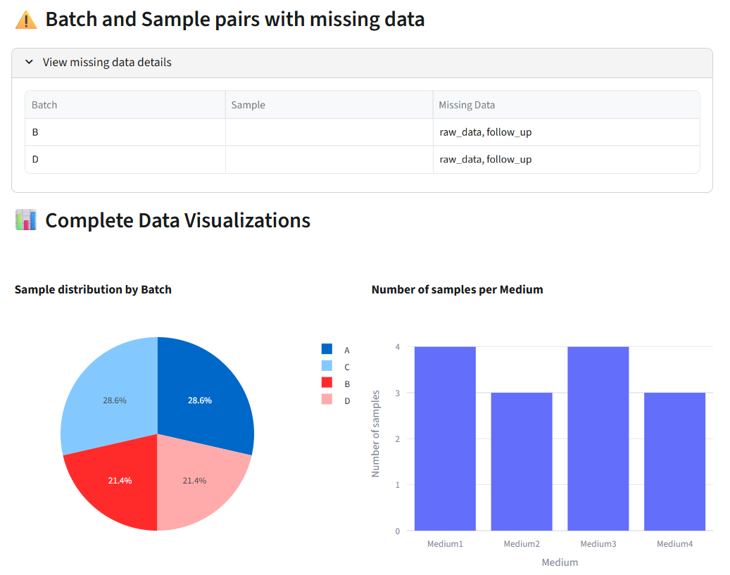
Key Actions:

• Verify all expected samples were loaded
• Identify which samples have missing data (info/raw_data/follow_up)
• Check batch and medium distribution
• Confirm data completeness before proceeding to selection

Selection

Interactive tool to select which batch-sample pairs you want to analyze.What you'll see:

• Existing Selections (if any):List of previously created selections with their ID and status
• Create New Selection:
• Interactive Data Table: Shows all valid samples (only complete data, no missing values)
• Columns displayed: Batch, Sample, Medium
• Multi-row selection mode: Click on rows to select/deselect
• Selected rows are highlighted

How to use:

1. Review the table of valid samples
2. Click on rows to select the batch-sample pairs you want to analyze
3. Click "Validate Selection" button to create a new selection scenario
4. The system launches a filtering scenario that creates a new ResourceSet with only selected samples

When to Use:

• Remove failed or problematic experiments from analysis
• Focus on specific batches or conditions
• Create multiple selections for comparison (e.g., "control group", "treatment group")
• Reduce dataset size for faster analysis

Output:

• New selection scenario created and launched
• Filtered ResourceSet containing only selected batch-sample pairs
• Selection saved with timestamp for future reference

🧪 Fermentor Selection

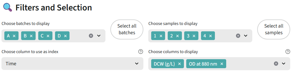
🧫 BiolectorXT Selection

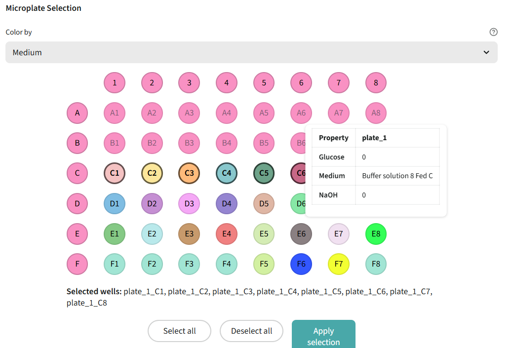
Table View

Browse your data in tabular format.

Features:

• Sortable and filterable columns
• Search functionality
• Export to CSV
• View metadata (batch, sample, medium composition)
• Pagination for large datasets

Graph View

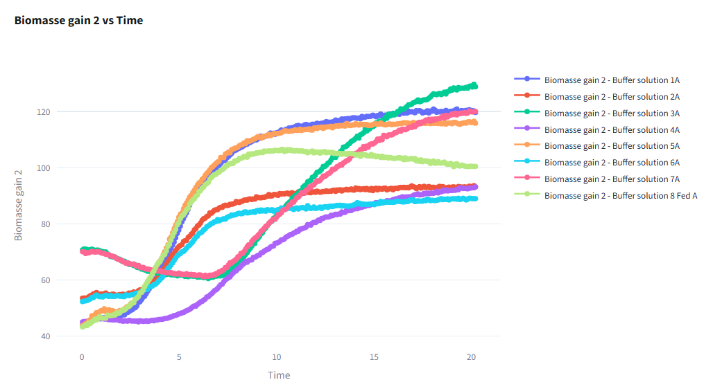
Visualize time series data with interactive plots.

Features:

• Multi-sample Plots: Compare multiple fermentation curves
• Parameter Selection: Choose which measurements to display (OD, pH, glucose, etc.)
• Color Coding: Automatically color by batch, sample, or medium type
• Interactive Zoom: Focus on specific time ranges
• Export Options: Download plots as PNG or SVG

Common Visualizations:

• Growth curves (OD vs Time)
• Substrate consumption
• Product formation
• pH evolution
• Multi-parameter overlay

Medium View

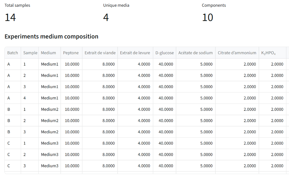
Explore and manage medium composition data.

Features:

• Medium Composition Table: View all medium formulations
• Compare Formulations: Side-by-side comparison of different media
• Import/Export: Upload new medium compositions or export existing ones
• Metadata Integration: Link medium data with fermentation results

Typical Use Cases:

• Document medium variations
• Identify formulation differences
• Prepare data for predictive analysis

Quality check

After visualizing your data, validate and clean it.

Features:

• Outlier Detection: Identify and remove statistical outliers using configurable thresholds
• Data Validation: Check for missing values, duplicates, and inconsistencies
• Visual Quality Reports:Distribution plotsTime series plots with outliers highlightedMissing data visualization
• Distribution plots
• Time series plots with outliers highlighted
• Missing data visualization
• Quality Metrics:Percentage of valid data pointsOutlier statistics per sampleData completeness scores
• Percentage of valid data points
• Outlier statistics per sample
• Data completeness scores

Configuration Options:

• Z-score threshold for outlier detection
• Minimum data points per sample
• Missing value handling strategies

Output: Cleaned and validated dataset ready for analysis

After the quality check, you will see a visualisation page again with the same functions as before, so you can inspect your data after applying the filters.

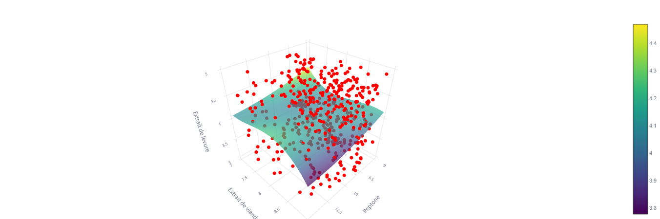
Medium PCA Analysis

Principal Component Analysis on medium composition data.

Purpose: Reduce dimensionality of medium composition data and identify key formulation patterns.

Features:

• Component Selection: Choose number of principal components (typically 2-3)
• Variance Explained: Understand how much variation each component captures
• 2D/3D Visualization: Interactive scatter plots colored by batches or outcomes
• Loadings Plot: See which medium components contribute most to each PC

Insights:

• Identify similar medium formulations
• Detect clustering patterns
• Understand which nutrients drive variability

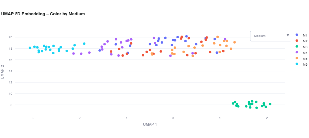
Medium UMAP Analysis

UMAP (Uniform Manifold Approximation and Projection) for medium composition.

Purpose: Non-linear dimensionality reduction for complex medium composition patterns.

Configuration:

• Number of Neighbors: Controls local vs global structure (default: 15)
• Minimum Distance: Affects point clustering tightness
• 2D/3D Output: Choose dimensionality for visualization
• K-Means Clustering: Optional automatic clustering

Advantages over PCA:

• Better preserves local structure
• More effective for non-linear relationships
• Clearer visual separation of groups

Results:

• Interactive 2D/3D plots
• Cluster assignments (if enabled)
• Downloadable coordinates table

Growth rate Analysis (Only for Biolector)

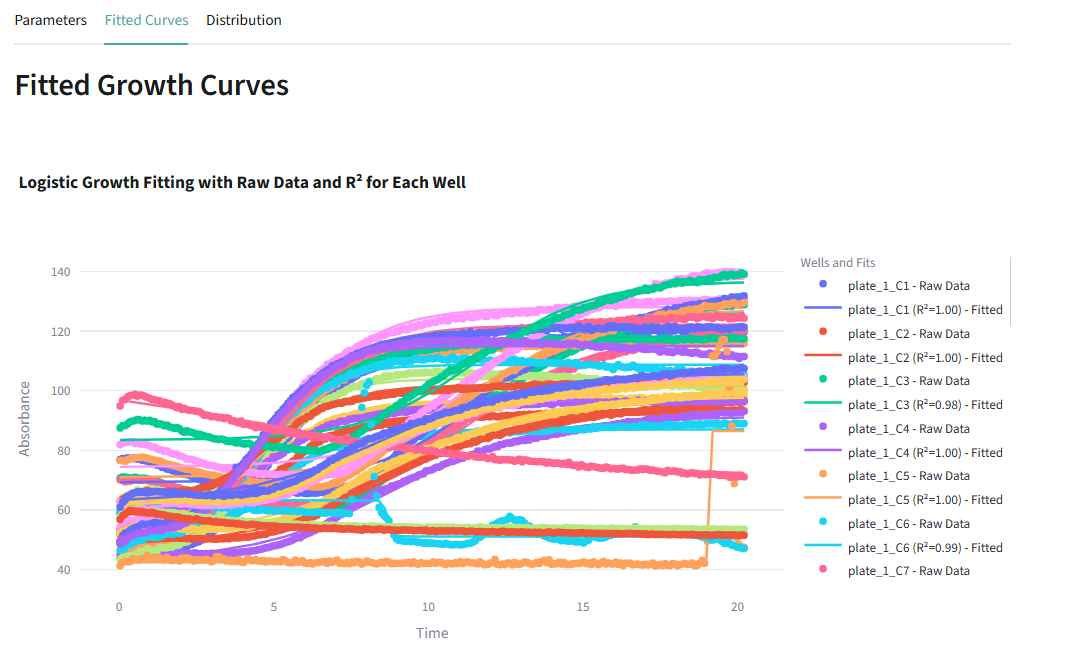
This page relates specifically to data from a Biolector.

Calculate growth rates and maximum absorbance values, and overlay raw data and fitted curves for precise insights.

Feature Extraction Analysis

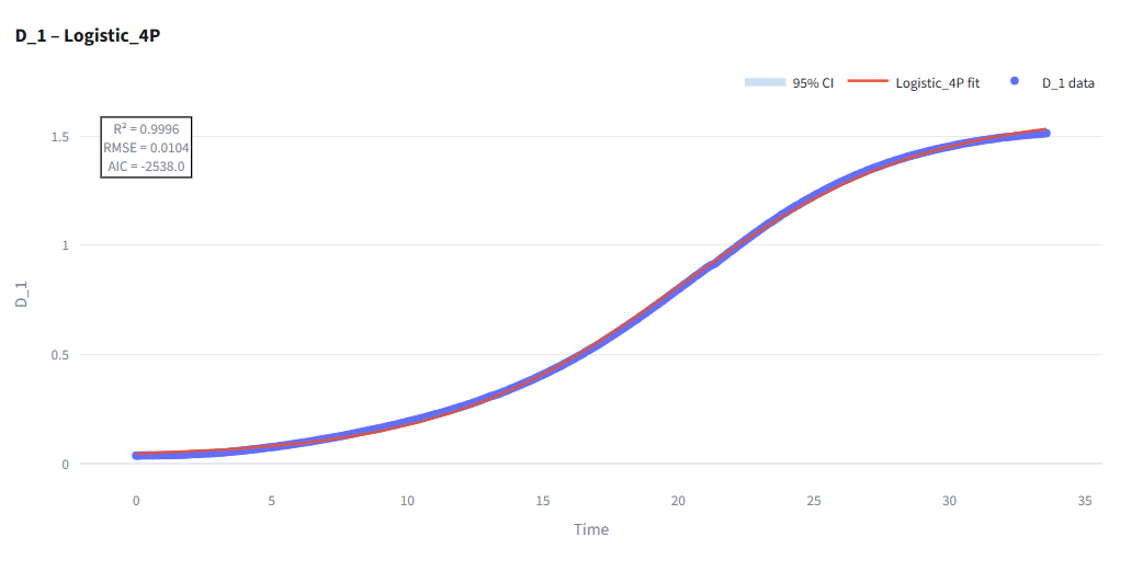
Extract biological characteristics from growth curves.

Purpose: Convert raw time-series data into biological features for predictive modeling.

Extracted Features:

• Growth Parameters:Maximum growth rate (μmax)Lag phase durationExponential phase durationMaximum OD reached
• Maximum growth rate (μmax)
• Lag phase duration
• Exponential phase duration
• Maximum OD reached
• Substrate Consumption:Consumption rateYield coefficients
• Consumption rate
• Yield coefficients
• Product Formation:Production rateFinal titerProductivity
• Production rate
• Final titer
• Productivity

Configuration:

• Select which parameters to extract
• Define calculation windows
• Choose smoothing methods

Output:

• Table with one row per sample
• Columns for each extracted biological feature
• Ready for machine learning analysis

Following analyses require the extracted features from Feature Extraction step to work properly. Make sure to run Feature Extraction before using these tools.  

Metadata Feature UMAP Analysis

Combine medium composition and extracted features for comprehensive UMAP analysis.

Prerequisites: Requires extracted features from Feature Extraction step.

Purpose: Visualize relationships between medium formulations and biological outcomes.

Features:

• Combined Dataset: Merges medium metadata with extracted features
• Column Selection: Choose which features to include in UMAP
• Medium Name Coloring: Color points by medium composition
• Hover Data: Display batch, trial, and other metadata on hover
• 2D/3D Visualization: Interactive plots with clustering option

Use Cases:

• Identify medium-performance relationships
• Find optimal formulation clusters
• Detect outlier experiments

PLS Regression

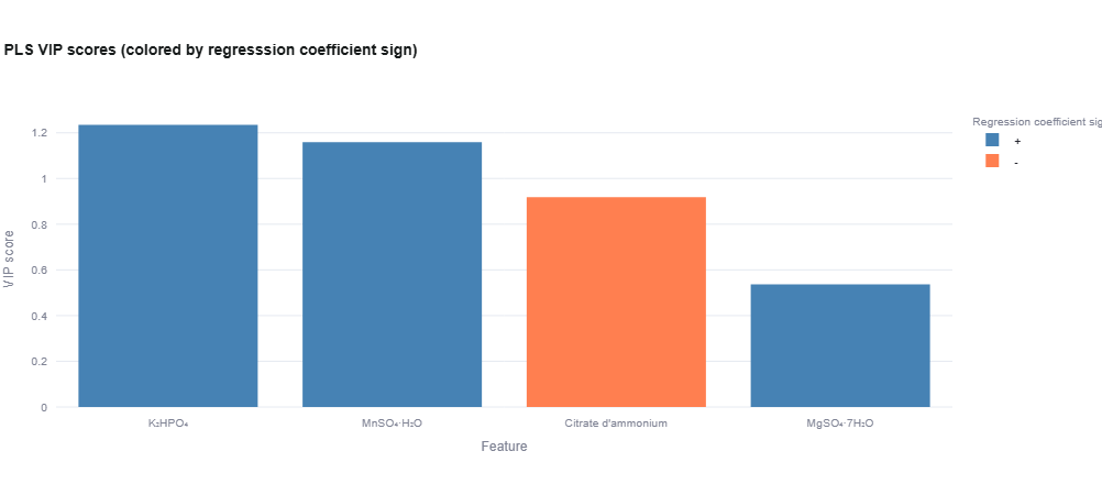
Partial Least Squares regression for predictive modeling.

Prerequisites: Requires extracted features from Feature Extraction step.

Purpose: Model relationships between medium composition (X) and biological characteristics (Y).

Workflow:

1. Select Target Variable: Choose which biological feature to predict (e.g., μmax, final titer)
2. Configure Model:Number of components (with cross-validation)Columns to exclude
3. Train Model: Automatic train/test split
4. Evaluate Results

Results Display:

• Performance Metrics:R² scoreRMSE (Root Mean Square Error)MAE (Mean Absolute Error)
• R² score
• RMSE (Root Mean Square Error)
• MAE (Mean Absolute Error)
• Predictions vs Actual: Scatter plots for train and test sets
• VIP Scores: Variable Importance in Projection (VIP > 1 = important)
• Component Selection: Cross-validation plot to choose optimal components

Advantages:

• Handles correlated predictors well
• Works with small sample sizes
• Provides interpretable variable importance

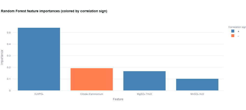
Random Forest Regression

Ensemble learning for non-linear predictive modeling.

Prerequisites: Requires extracted features from Feature Extraction step.

Purpose: Predict biological characteristics using decision tree ensembles.

Configuration:

• Number of Trees: More trees = better stability (default: 100)
• Maximum Depth: Controls tree complexity (None = no limit)
• Random Seed: For reproducibility
• Target Variable: Which biological feature to predict
• Feature Selection: Choose which medium components to include

Results Display:

• Performance Metrics: R², RMSE, MAE
• Feature Importance: Bar chart showing which medium components matter most
• Predictions vs Actual: Train and test set visualizations
• Top 10/20 Important Variables: Tables with importance scores

When to Use:

• Non-linear relationships expected
• Large feature sets
• Need robust predictions
• Want feature importance rankings

Causal Effect

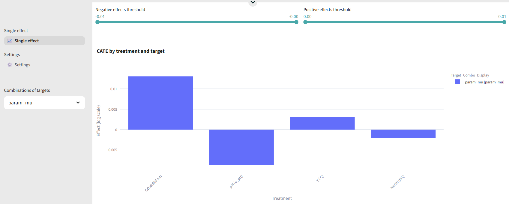
Identify cause-and-effect relationships between medium components and outcomes.

Purpose: Go beyond correlation to understand causal relationships.

Methods:

• Causal inference algorithms
• Intervention analysis
• Counterfactual reasoning

Features:

• Causal graph visualization
• Effect size estimation
• Confidence intervals

Output:

• Directed causal graphs
• Effect magnitude tables
• Recommendations for medium optimization

Optimization

Use genetic algorithms to find optimal medium composition.

Purpose: Automatically discover the best medium formulation to maximize biological performance.

Configuration:

1. Constraints Resource: Upload JSON file with component bounds{ "glucose": {"lower_bound": 0, "upper_bound": 20}, "nitrogen": {"lower_bound": 0.5, "upper_bound": 5} }
2. Optimization Parameters:Population size (default: 50)Number of iterations (default: 100)
3. Targets and Objectives:Define which features to optimize (e.g., μmax, final titer)Set minimum acceptable values for each targetAdd multiple targets (multi-objective optimization)

Algorithm:

• Genetic algorithm with mutation and crossover
• Pareto optimization for multi-objective cases
• Constraint handling

Results:

• Optimal medium formulation(s)
• Predicted performance values
• Convergence plots
• Sensitivity analysis

Use Cases:

• Design of Experiments (DoE) follow-up
• Medium formulation development
• Cost reduction while maintaining performance
• Multi-parameter optimization

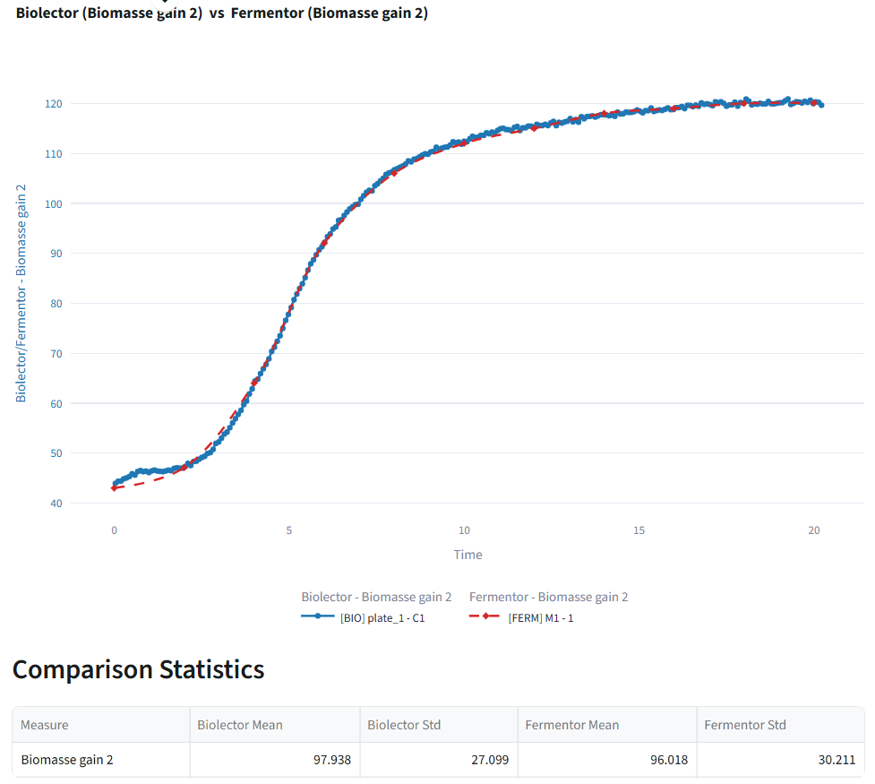
🔎 Biolector/Fermentor Comparison

Once a Comparison recipe is runned, you can compare the performance of Biolector and fermentor experiments for the same process. 

You will see : 

• Comparison plot displaying Biolector and fermentor data on the same graph.
• Summary statistics for each dataset, including:
• Mean
• Standard deviation

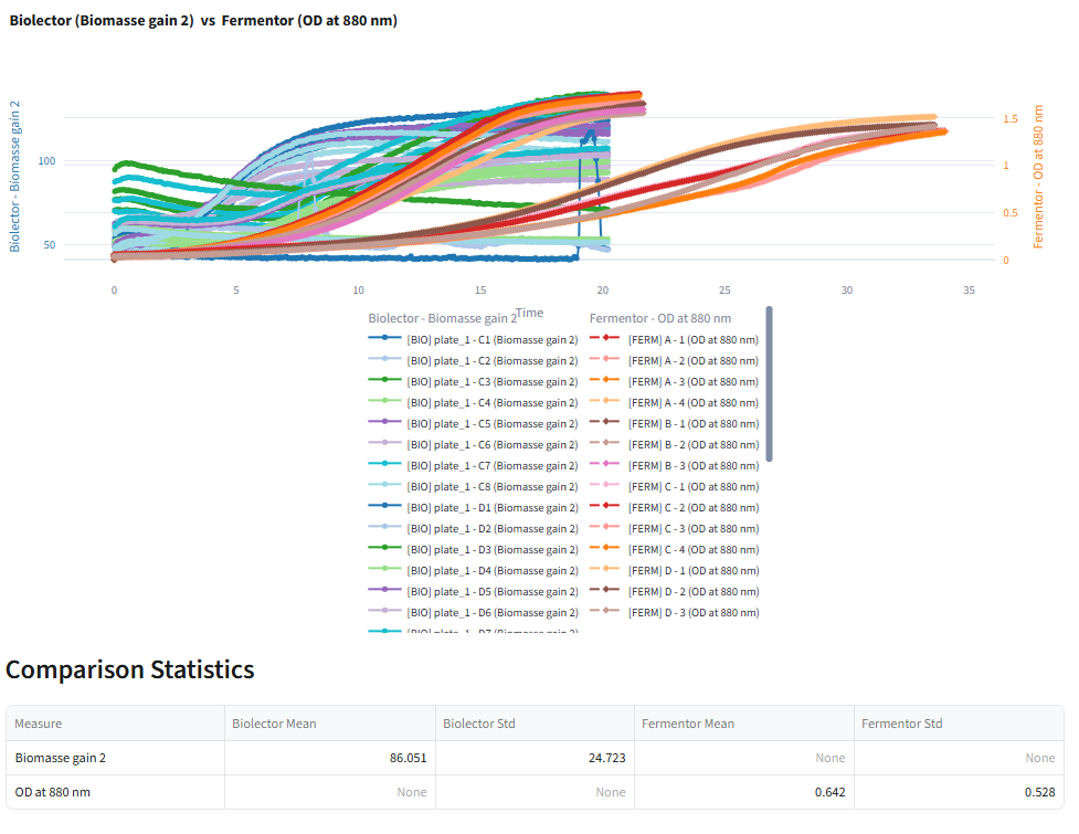
You are now ready to make sense of your bioprocess data and manage your experiments more effectively! 

Tips and Best Practices

Data Preparation

• Ensure consistent column naming across files
• Check for missing values before analysis
• Document medium compositions clearly
• Use meaningful batch and sample names

Selection Strategy

• Create multiple selections for comparison (e.g., "good batches", "failed batches")
• Keep a "full dataset" selection for reference
• Select only valid samples (complete data)

Visualization & Quality Control

• Visualize data first to identify potential issues
• Always run Quality Check after visualization
• Review outlier detection results manually
• Document why specific samples are excluded
• Export quality reports for documentation

Analysis Workflow

• Start with exploratory analysis (PCA/UMAP) before modeling
• Extract features before running predictive models
• Use PLS for initial modeling, Random Forest for complex relationships
• Validate models with train/test splits

Optimization

• Start with wide constraint ranges, then narrow
• Use multiple optimization runs with different random seeds
• Validate optimization results experimentally
• Consider cost constraints in multi-objective optimization

Common Issues and Solutions

Problem: "No data available"

Solution: Check that Selection step completed successfully and produced a valid ResourceSet.

Problem: "Analysis failed"

Solution:

• Verify input data has required columns
• Check for missing values in critical columns
• Ensure numeric columns are properly formatted

Problem: "Model performance is poor"

Solution:

• Increase number of samples (minimum 20-30 recommended)
• Check for outliers in data
• Try different feature sets
• Consider data normalization

Problem: "Optimization doesn't converge"

Solution:

• Increase population size or iterations
• Check constraint bounds are reasonable
• Verify target objectives are achievable
• Review quality of training data

How to delete a recipe?

To delete a recipe, go to the first scenario (the one containing the load data task) and click 'Delete scenario'. This will delete the associated scenario and, consequently, the recipe.

Export and Reporting

All analysis steps provide export options:

• CSV Downloads: Tables, coordinates, metrics
• Plot Exports: PNG, SVG formats
• Scenario Reports: Complete analysis documentation
• Model Artifacts: Save trained models for reuse