gws_omix

Introduction

Ever since the beginning of the 21st century, we have witnessed remarkable technological advancements in biology, particularly with the emergence of high-throughput ‘omics’ techniques such as microarrays and next-generation sequencing (NGS). These approaches revolutionized genomics by enabling the simultaneous measurement of thousands of genes in a single experiment. As a result, researchers can now rapidly identify genes whose expression is associated with particular phenotypes, treatments, or conditions.

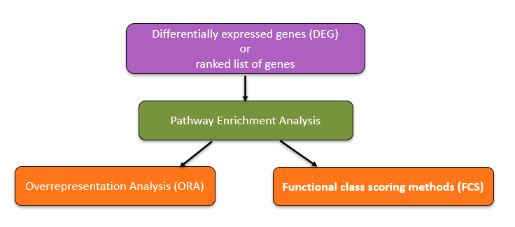
However, identifying differentially expressed genes (DEGs) is only the first step. The true challenge lies in interpreting these long gene lists in a biologically meaningful way. A list of hundreds or thousands of genes provides little insight on its own; instead, scientists need to understand which biological processes, pathways, or molecular mechanisms are perturbed. To address this challenge, a variety of computational approaches have been developed to translate raw gene-level information into interpretable functional categories. This family of approaches is collectively known as Pathway Enrichment Analysis (PEA) 

The central aim of FEA is to determine whether certain biological annotations such as pathways, molecular functions, or cellular components are statistically overrepresented in a gene set of interest relative to an appropriate reference background. By linking DEGs to known biological knowledge bases (e.g., Gene Ontology (GO), KEGG pathways, or Reactome), FEA allows researchers to move from raw lists of genes to higher-level interpretations about the underlying biological mechanisms in their study system.

ORA = I have a shortlist => is this pathway overrepresented in it?

GSEA = Across the whole ranked list => do the genes from a pathway cluster toward the top or the bottom?

If you’re new to ORA, this short video explains the core idea behind Overrepresentation Analysis and how to interpret its results: (click here) 

If you’re new to GSEA, this short video explains the core idea behind Gene Set Enrichment Analysis and how to interpret its results: (click here) 

Methods

1.   Overrepresentation Analysis (ORA)

1.1  What's ORA?

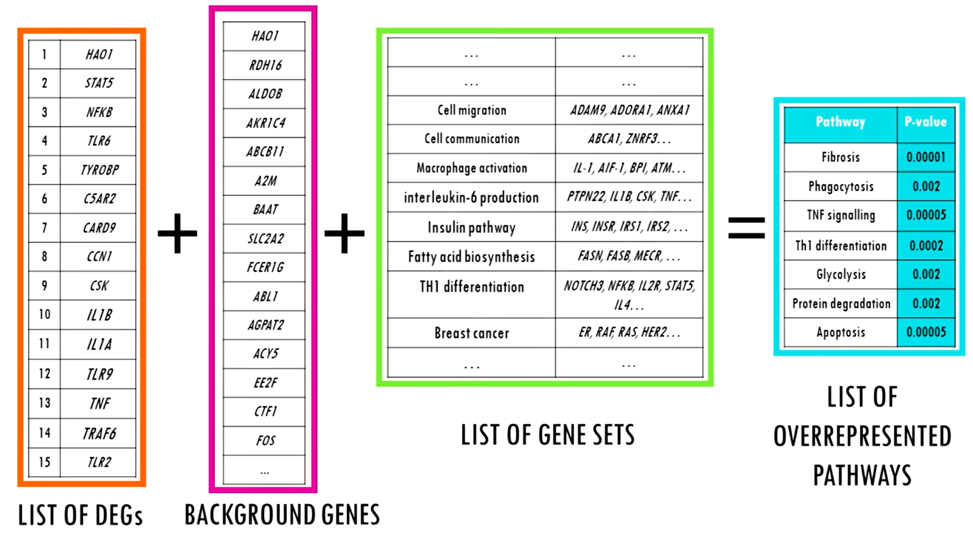
ORA is one of the most widely used and conceptually simple methods for functional enrichment. Here, the input is a discrete list of genes typically DEGs identified after applying thresholds on adjusted p-values and fold-changes.

The question ORA asks is:

Do certain pathways or functional categories contain more genes from my list than would be expected by chance?

This is statistically tested using the hypergeometric test, which assesses whether the overlap between the gene list and a given pathway is greater than random expectation.

 One important consideration in ORA is the definition of the background universe. By default (auto mode), the background is set to the entire reference genome (e.g., ~20,000 genes in humans). Alternatively, in experiment mode, the background can be defined as all genes tested in the experiment (e.g., ~12,000 measured transcripts in RNA-seq). The choice of background influences the results, especially in tissue or platform specific datasets.  

1.2 Tools

While several popular R packages exist for functional enrichment analysis, such as topGO and clusterProfiler, the g:Profiler ecosystem (including the R client gprofiler2) offers distinct advantages. Unlike tools that require local downloads of multiple annotation databases, g:Profiler provides access to a broad range of high-quality, regularly updated annotation sources through a single query. Its in-house database integrates only well-established and reliable resources, including Gene Ontology (GO), KEGG, Reactome, WikiPathways, miRTarBase, TRANSFAC, the Human Protein Atlas, protein complexes from CORUM, and the Human Phenotype Ontology.

Another important feature is its automatic identifier mapping: g:Profiler seamlessly handles input lists containing mixed types of gene identifiers (e.g., Ensembl IDs, gene symbols, Entrez IDs), removing a common source of preprocessing errors. This flexibility, combined with continuous updates and support for over 600 species and strains, makes g:Profiler an ELIXIR Recommended Interoperability Resource in life sciences. Overall, g:Profiler provides a user-friendly, reproducible, and comprehensive framework for conducting functional enrichment analysis without the technical burden of managing multiple annotation sources locally.

1.3 Steps

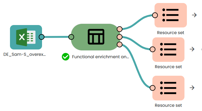
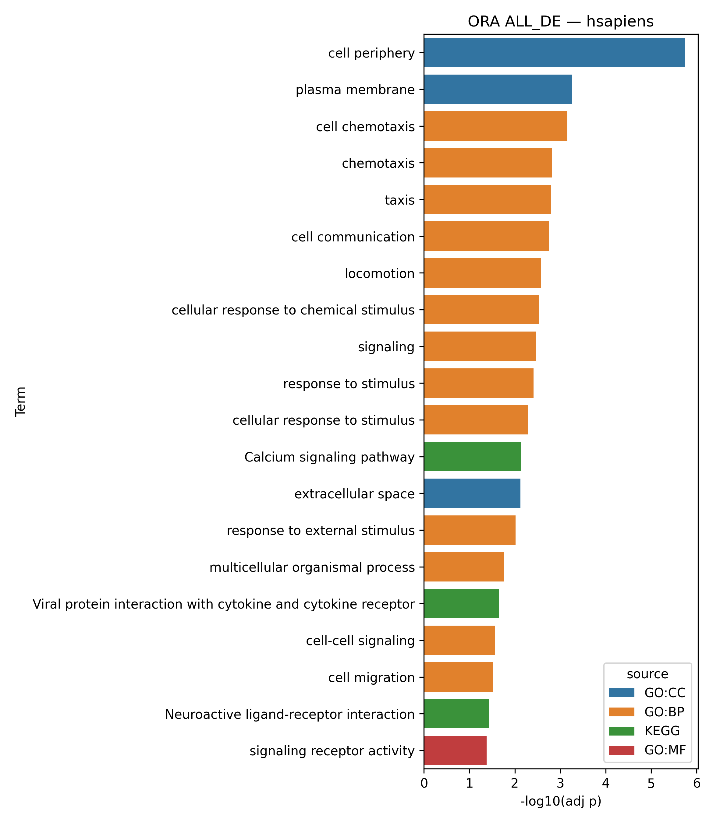
This task (task: OmiX – Functional enrichment analysis based on ORA) performs functional enrichment analysis on the list of differentially expressed genes (DEGs). It conducts Over-Representation Analysis (ORA) using a hypergeometric/Fisher’s exact test, followed by multiple-testing correction (by default via g:SCS – Set Counts and Sizes).

In this workflow, the background universe is set to auto (the whole genome as defined by g:Profiler) rather than experiment (all genes quantified in the dataset). This choice ensures consistency with the g:Profiler web interface, where only terms passing the corrected significance threshold (adjusted p-value ≤ α) are retained.

🧰 Prerequisites

• Access to Constellab and a valid Digital Lab environment
• Installed bricks: gws_omix ≥ 0.13.15

Parameters:

Outputs

2.   Functional class scoring methods (FCS)

       2.1    Gene set enrichment analysis (GSEA)

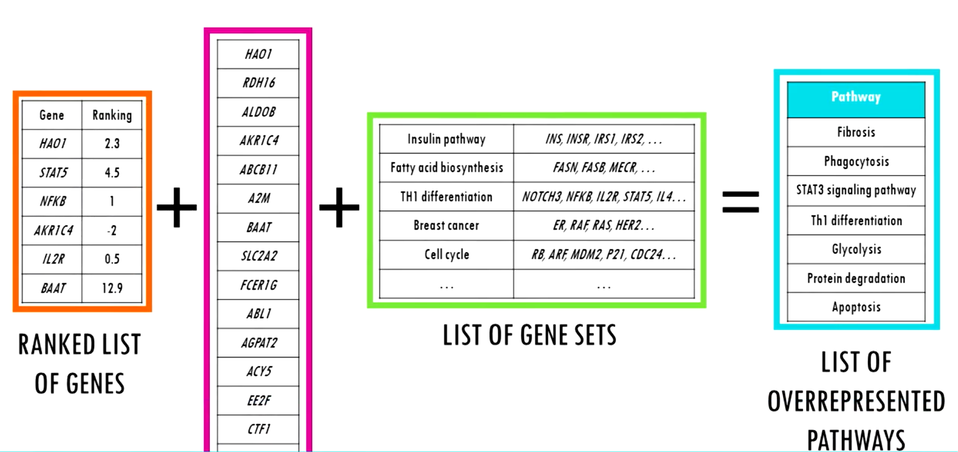
Gene set enrichment analysis (GSEA) is a widely used, knowledge-based approach for interpreting genome-wide expression or ranking data by testing whether members of a predefined gene set tend to occur toward the top or bottom of a ranked gene list, rather than focusing on single genes in isolation. This shift in perspective is especially useful when biologically coherent but individually modest expression changes are distributed across many genes, a scenario in which gene-by-gene testing can miss coordinated signals. The original GSEA framework introduced a running-sum enrichment score that quantifies the degree to which a gene set is over-represented at the extremes of the ranked list, and assesses significance via permutation to account for correlation structure and multiple testing considerations.

https://pubmed.ncbi.nlm.nih.gov/16199517/ 

🧰 Prerequisites

• Access to Constellab and a valid Digital Lab environment
• Installed bricks: gws_omix ≥ 0.13.15

1. Purpose

GSEAEnrichmentGMT runs pre-ranked GSEA from:

• a results table containing a gene identifier column and a signed ranking statistic (the input should be the raw, unfiltered output table produced by the “pyDESeq2 multi-contrast” task for example. => Do not use filtered/significant-only tables.
• a GMT file describing gene sets (pathways / GO terms / modules).

What is a GMT?

A GMT (Gene Matrix Transposed) file is a simple gene-set format where each line is one gene set:

GeneSetNameDescriptionGene1Gene2...

So a GMT is basically a collection of pathways/terms, each represented as a list of genes.

It produces:

• per-gene-set results table (NES, p-value, etc.),
• a long “gene × gene set” table (for the interactive grid),
• PNG figures (top-20 barplot + enrichment plots),
• two ResourceSets: results: tables + grid + non-enrichment figures, enrichplots: enrichment plot PNGs only.

2. Computation method (pre-ranked GSEA)

2.1 Ranked list preparation

From the input table, the task reads:

• genes_colname: gene identifiers,
• stat_colname: signed ranking statistic.

Cleaning and ranking:

• numeric conversion of the stat column,
• drop invalid rows,
• handle duplicate genes by keeping the entry with maximum |stat|,
• sort descending by stat (highest ranked first).

2.2 GSEA computation with GSEApy prerank

The core analysis uses GSEApy prerank. Key parameters:

• permutation_num (nperm): number of permutations (smallest nominal p-value ≈ 1/nperm).
• min_size, max_size: filter gene sets by overlap size with the ranked list.
• processes: parallel execution.

2.3 Reported statistics

Typical outputs per gene set:

• ES: enrichment score,
• NES: normalized enrichment score,
• p_value: nominal permutation p-value,
• qvalue/FDR if provided by GSEApy,
• padj: BH-adjusted p-values computed by the task (FDR control).

3. “Top N enrichment plots” (n_enrichplots)

3.1 What n_enrichplots does

n_enrichplots controls how many classic enrichment plots are generated as PNG files:

• GSEA_enrichment_01_<TERM>.png … GSEA_enrichment_NN_<TERM>.png.

3.2 How “Top” terms are selected

Selection follows “most significant first, then strongest effect”:

1. significance metric priority:

• qvalue if available,
• else padj (BH),
• else p_value (nominal).

1. tie-breaker:

• sort by |NES| descending.

So the plotted top N gene sets are chosen by (qvalue or padj or p_value) ascending, then |NES| descending.

4. Parameters (ConfigSpecs)

• genes_colname (default: "gene"): gene identifier column name.
• stat_colname (default: "stat"): signed ranking statistic column.
• min_size (default: 15): minimum overlap size after filtering.
• max_size (default: 500): maximum overlap size.
• nperm (default: 1000 in your script): number of permutations (p-value floor ≈ 1/nperm).
• processes (default: 4): parallel workers.
• n_enrichplots (default: 10): number of enrichment PNG plots to generate.
• grid_genes_per_page (default: 25) and grid_sets_per_page (default: 20): pagination controls for the interactive grid.

5. Inputs

• de_table_file (Table or File): must contain genes_colname and stat_colname.
• gmt_file(File): GMT file, one gene set per line:set_id<TAB>description<TAB>gene1<TAB>gene2...

6. Outputs

The task returns two ResourceSets:

6.1 results ResourceSet

Contains:

• GSEA_results.csv imported as a Table
• GSEA_matrix_long.csv imported as a Table
• non-enrichment PNG figures (e.g., GSEA_top20_barplot.png)
• an interactive Plotly grid built from GSEA_matrix_long.csv

6.2 enrichplots ResourceSet

Contains only:

• GSEA_enrichment_*.png

FAQ

From ORA to GSEA: why ranking-based enrichment?

Pathway enrichment methods aim to summarize gene-level results into higher-level biological interpretations. Instead of interpreting hundreds or thousands of genes one by one, they test whether genes belonging to a given pathway (gene set) show a non-random pattern in the experiment.

In Over-Representation Analysis (ORA), the input is a shortlist of genes (typically DEGs after applying thresholds such as adjusted p-value and |log2FC|). For each pathway, ORA asks whether the overlap between the pathway genes and the DEG list is greater than expected by chance (commonly using a hypergeometric or Fisher’s exact test), followed by multiple-testing correction across many pathways. Lower adjusted p-values indicate that the observed overlap is unlikely under the null model.

A key limitation of ORA is its dependence on arbitrary DEG thresholds. Genes close to the cutoffs (e.g., |FC| just below the threshold or adjusted p-value just above it) may still carry consistent biological signal, yet they are excluded from the analysis. This can noticeably change the enrichment results, especially when the number of significant DEGs is small.

To reduce this sensitivity to hard thresholds, a “second generation” of enrichment methods was introduced: Functional Class Scoring (FCS) approaches. Rather than requiring a discrete DEG list, FCS methods use all genes and test whether genes from a pathway tend to accumulate toward the top or bottom of a ranked gene list.

Gene Set Enrichment Analysis (GSEA) is the best-known FCS method. Its input is a ranked list of all genes, ordered by a ranking metric that reflects association with the phenotype (the exact metric depends on the differential expression method or study design). GSEA then evaluates whether pathway genes are enriched at the extremes of that ranked list, rather than being overrepresented in a pre-selected DEG subset.

What is a GAF, and why is it useful for GSEA?

A GAF (Gene Association File) is a standard tab-delimited file distributed by the Gene Ontology consortium that lists gene → GO term annotations, including evidence codes (like IEA) and GO aspects (BP/MF/CC). It’s essentially a big catalog of which genes are associated with which GO terms. (https://pmc.ncbi.nlm.nih.gov/articles/PMC6377150/) 

GSEA does not take a GAF directly. Instead, you use a GAF to build a GMT, and that GMT is what GSEA consumes.

Why GAF helps in your pipeline:

• Many species don’t have ready-made pathway gene sets in GMT form.
• But they may have GO annotations available as GAF.
• So your GAF → GMT task turns those GO annotations into gene sets usable by GSEA.

Official places to download GAFs are provided by the GO consortium (https://current.geneontology.org/products/pages/downloads.html?).

In your GO case:

• Each GO term (e.g., “mitochondrial translation”) becomes a gene set.
• The genes annotated to that GO term become the members of that gene set.
• You can generate separate GMTs by GO aspect: BP = Biological Process MF = Molecular Function CC = Cellular Component and also an ALL version that mixes aspects

Your GAF→GMT task outputs multiple GMT variants (BP/MF/CC/ALL, withIEA/noIEA, id/symbol) so users can pick the version that matches their gene identifiers and strictness needs.

What is IEA?

IEA = Inferred from Electronic Annotation. It means the gene → GO term association was assigned automatically by a computational pipeline (rules, sequence similarity, protein domains, etc.), without human curator review of each annotation.

In plain terms: “a computer pipeline assigned this GO term to this gene.” IEA is used for inferences made without human supervision.

source : https://pmc.ncbi.nlm.nih.gov/articles/PMC6377150/

What does “noIEA” mean?

noIEA is not an official GO evidence code. It’s a practical option meaning.

So:

• withIEA = keep IEA + everything else
• noIEA = keep everything else except IEA

Why does this option exist?

Because IEA annotations come with a classic trade-off:

withIEA (include IEA)

• ✅ Much higher annotation coverage → more genes annotated, especially in less-studied species
• ✅ More “filled” gene sets → GSEA has more usable sets
• ⚠️ Potentially more noise / less specificity depending on the pipeline

noIEA (exclude IEA)

• ✅ More conservative: you keep annotations with stronger curator oversight / stronger traceability
• ✅ Lower risk of overly broad automated inferences
• ⚠️ Lower coverage → sometimes reduced power for GSEA (fewer sets, sets too small, etc.)

source:  https://pmc.ncbi.nlm.nih.gov/articles/PMC3364937/