Introduction

Supervised learning (SL) is a machine learning approach that addresses problems where labeled data is available. In this paradigm, each data point consists of features (covariates) and a corresponding label. The objective of supervised learning algorithms is to learn a function that can map input feature vectors to their respective labels, using the provided example input-output pairs. These algorithms infer the function by analyzing a set of labeled training data, which comprises training examples. Each training example consists of an input object, usually a vector, and a desired output value known as the supervisory signal. The supervised learning algorithm examines the training data to generate an inferred function that can be applied to new, unseen examples. Ideally, the algorithm should accurately assign class labels to unseen instances. Achieving this requires the learning algorithm to generalize from the training data in a reasonable manner.

Steps to follow

To address a supervised learning problem effectively, the following steps should be followed:

1. Identify the nature of the training examples: Determine the specific type of data that will be used as the training set. For instance, in the case of handwriting analysis, the training examples could be individual handwritten characters, entire words, sentences, or even paragraphs.
2. Gather a representative training set: Collect a training set that accurately represents the real-world scenarios in which the learned function will be applied. This set should consist of input objects and their corresponding outputs, obtained either from human experts or through measurements.
3. Determine the input feature representation: The accuracy of the learned function heavily relies on how the input objects are represented. Typically, input objects are transformed into feature vectors that contain descriptive features. It is crucial to strike a balance, ensuring that the number of features is not excessively large (to avoid the curse of dimensionality) while still providing sufficient information to make accurate predictions.
4. Determine the structure of the learned function and the appropriate learning algorithm: Choose the suitable learning algorithm and the corresponding structure for the learned function. For example, options may include support-vector machines or decision trees, depending on the problem at hand.
5. Finalize the design: Apply the chosen learning algorithm to the gathered training set. Some algorithms require specific control parameters that need to be determined. These parameters can be adjusted by optimizing performance on a subset called a validation set, or through techniques like cross-validation.
6. Evaluate the accuracy of the learned function: After the learning process and parameter adjustments, assess the performance of the resulting function using a separate test set. This test set should be distinct from the training set and serves as an independent measure of the function's effectiveness.

By following these steps, one can systematically approach a supervised learning problem, ultimately developing a reliable and accurate learned function for practical use.

Logistic regression

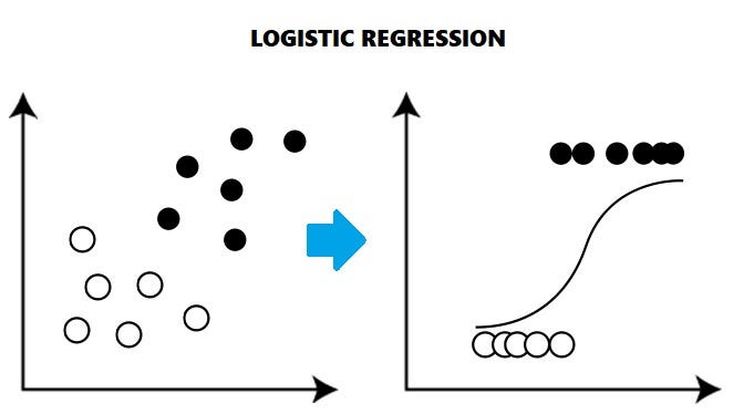
Logistic regression is a statistical method commonly used by biologists to analyze and predict binary or categorical outcomes in biological research. It is particularly useful when studying factors that influence the occurrence or probability of an event, such as disease presence or absence, survival rates, or response to a treatment.

In logistic regression, the dependent variable is binary (e.g., presence or absence of a disease), and the independent variables are typically continuous or categorical variables (e.g., age, gender, genetic markers). The goal is to estimate the relationship between the independent variables and the probability of the binary outcome.

The logistic regression model uses the logistic function, also known as the sigmoid function, to transform a linear combination of the independent variables into a predicted probability value between 0 and 1. This predicted probability represents the likelihood of the event occurring.

During the model training process, the logistic regression algorithm calculates the optimal coefficients (weights) for each independent variable, aiming to maximize the likelihood of the observed data. These coefficients indicate the direction and magnitude of the impact each independent variable has on the outcome. Once the model is trained, it can be used to predict the probability of the binary outcome for new observations based on their independent variables. A threshold can be set to classify observations into different categories (e.g., above or below a certain probability value).

In biology, logistic regression can be applied in various contexts. For example, it can be used to analyze the association between genetic markers and the risk of developing a disease, or to investigate the influence of environmental factors on the presence of a particular species in a habitat. Logistic regression allows biologists to assess the significance and strength of these relationships, providing valuable insights for understanding and predicting biological phenomena.

The k-nearest neighbors (k-NN)

The k-nearest neighbors (k-NN) algorithm is a machine learning technique commonly used by biologists to analyze and classify biological data based on similarity. It is a non-parametric method that can be applied to both categorical and continuous variables.

In the k-NN algorithm, the data points are represented as vectors in a multi-dimensional space, with each dimension corresponding to a specific feature or attribute. When a new data point is to be classified, the k-NN algorithm finds the k nearest neighbors to that data point based on a distance metric (e.g., Euclidean distance or Manhattan distance). The value of k is a user-defined parameter.

Once the k nearest neighbors are identified, the algorithm assigns a class label to the new data point based on the majority class among its neighbors. For example, if the majority of the k nearest neighbors belong to a certain category, the algorithm will classify the new data point into that category.

The choice of k is important as it influences the decision boundary and classification accuracy. A smaller value of k may result in a more flexible decision boundary, but it can also be sensitive to noise and outliers. On the other hand, a larger value of k may lead to a smoother decision boundary but could potentially overlook local patterns or variations.

In a biological context, k-NN can be applied to various tasks. For instance, it can be used to classify biological samples based on gene expression profiles, where the gene expression levels serve as the features. By considering the k nearest neighbors with known classifications, the algorithm can predict the class or phenotype of a new sample.

Additionally, k-NN can be used for species identification, where morphological or genetic features are used as input. By comparing the features of an unknown specimen to those of the k nearest neighbors in a reference dataset, the algorithm can assign a species label to the specimen.

Overall, k-NN provides a simple yet effective method for classification and pattern recognition in biological data analysis. By leveraging the concept of proximity and similarity, it enables biologists to make predictions and gain insights from their data based on the characteristics of similar instances in the dataset.

Support Vector Machine and derivative

Support Vector Regression (SVR), Support Vector Machine (SVM), and Support Vector Classification (SVC) are machine learning algorithms commonly used by biologists for various analytical tasks. They are part of the broader family of Support Vector Machines (SVM), which is a powerful and versatile class of algorithms for both regression and classification problems.

Support Vector Regression (SVR) is primarily used for regression tasks in biology. It aims to build a model that can accurately predict continuous or numerical outcomes based on input features. SVR works by finding a hyperplane in a high-dimensional feature space that maximally fits the training data while controlling the error or deviation within a certain tolerance level. The hyperplane represents the regression function, and the support vectors are the training data points that lie closest to the hyperplane. SVR handles non-linear relationships by mapping the input features into a higher-dimensional space using kernel functions, allowing for more complex and flexible regression models.

Support Vector Machine (SVM) and Support Vector Classification (SVC) are employed when the objective is to perform binary or multi-class classification tasks in biology. SVM and SVC aim to find an optimal hyperplane that effectively separates different classes or categories in the feature space. The hyperplane is chosen to maximize the margin, which is the distance between the hyperplane and the nearest training data points of different classes. The support vectors, again, are the data points closest to the hyperplane. SVM and SVC can handle non-linear classification problems by utilizing kernel functions, which transform the feature space to a higher-dimensional representation, enabling the creation of non-linear decision boundaries.

In biology, these algorithms find application in various scenarios. For instance, SVR can be used to predict quantitative biological properties such as protein folding rates, gene expression levels, or enzyme activity based on relevant features. SVM and SVC can be utilized for tasks like disease classification based on genetic or biomarker data, identifying species based on morphological or genomic features, or predicting drug response based on patient characteristics.

These algorithms provide robust and effective tools for analyzing biological data, as they can handle complex relationships and high-dimensional feature spaces. They are widely used in bioinformatics, genomics, proteomics, and other fields to extract meaningful patterns and make accurate predictions, ultimately contributing to advancements in biological research and applications.

Random Forest

Random Forest is a supervised machine learning algorithm that combines multiple decision trees to create a more robust and accurate model. Here's a brief explanation of how the Random Forest Classifier works:

1. : A decision tree is a flowchart-like structure where each internal node represents a feature or attribute, each branch represents a decision rule, and each leaf node represents the outcome or class label. Decision trees make decisions based on the feature values and recursively split the data into subsets.

1. : Random Forest Classifier combines multiple decision trees, creating an ensemble. Each tree is built on a random subset of the training data (random sampling with replacement, known as bootstrap aggregating or "bagging"). Additionally, at each node of each tree, only a random subset of features is considered for splitting, reducing the correlation between trees.

1. : During the classification process, each decision tree in the Random Forest independently predicts the class label based on its structure and the input features. The class prediction is determined by majority voting among the individual trees. The final class label is the one with the most votes.

Random Forest Classifier offers several benefits, including:

• Robustness against overfitting: By constructing an ensemble of diverse decision trees and aggregating their predictions, Random Forest reduces the risk of overfitting compared to individual decision trees.
• Feature importance: Random Forest can estimate the importance of different features in the classification task, providing insights into the most influential factors.
• Versatility: It can handle both categorical and numerical features and is suitable for various classification problems.