Introduction
One of the most cost-effective and rapid genomic approaches to determining the species composition of a microbiome is to sequence one or more genes (called barcodes or tags) common within the living kingdom. For example, sequencing the gene coding for 16S rRNA will reveal the representation and abundance of different bacterial species present in samples. The reads obtained after sequencing are aligned with bacterial genomes referenced in databases, allowing the identification and taxonomic classification of the sequenced species.
Data upload and preparation
Input fastq folder
One must upload one folder with all the sequencing data using the
. You must select the following format: Fastq folder.
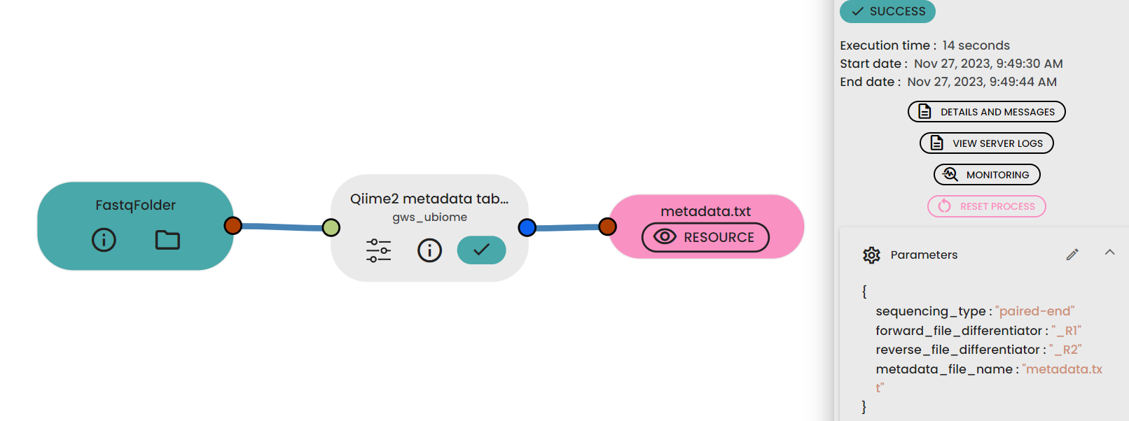
Generation of the metadata file
The uBiome Make metadata file task automatically generates a ready-to-use metadata file using ( task: uBiome -Qiime2 metadata table maker) when given a fastq folder as input. Once the metadata file is generated,
in the expected file format (see below).
Exemple :
#author: Paulson, Robert
#data: 1996/08/17
#project: Chaos
#types_allowed:categorical or numeric
#column-type	categorical	categorical	categorical
sample-id	forward-absolute-filepath	reverse-absolute-filepath	status
Sample_1	Sample_1.forward.fq.gz	Sample_1.reverse.fq.gz	ctrl
Sample_2a	Sample_2a.forward.fq.gz	Sample_2a.reverse.fq.gz	T1
Sample_2b	Sample_2b.forward.fq.gz	Sample_2b.reverse.fq.gz	T1
Sample_3a	Sample_3a.forward.fq.gz	Sample_3a.reverse.fq.gz	T2
Sample_3b	Sample_3b.forward.fq.gz	Sample_3b.reverse.fq.gz	T2
Protocol
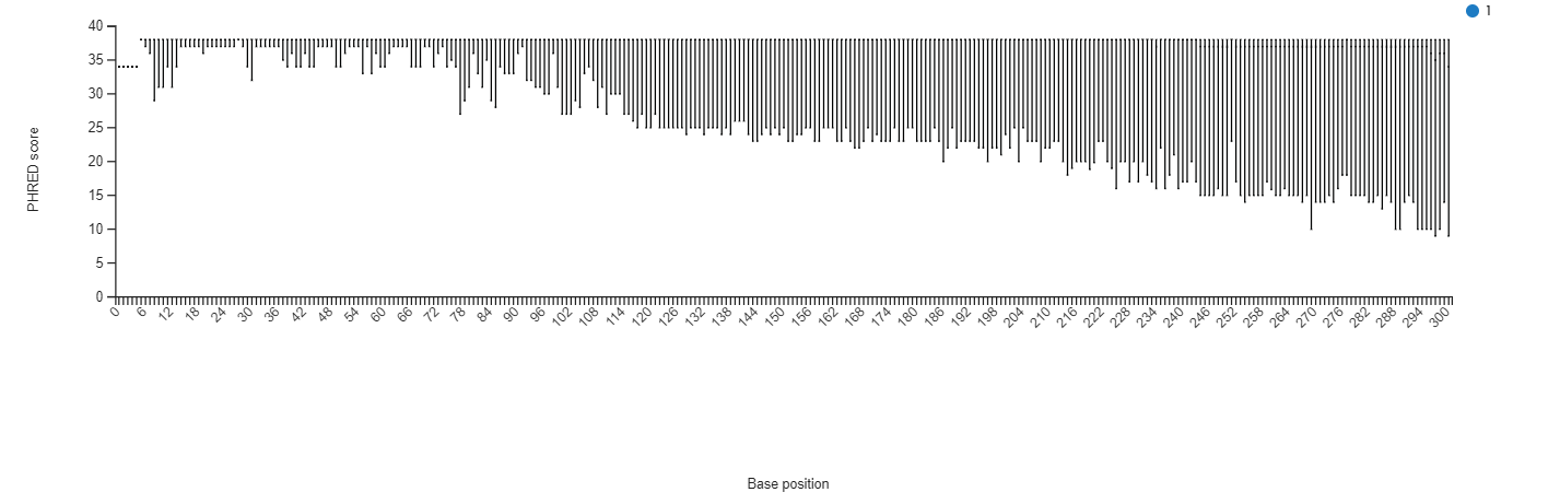
STEP 1 - Checking the reads quality
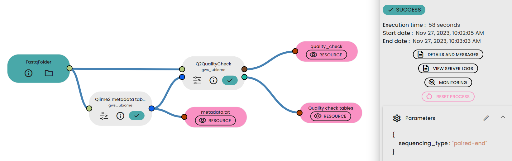
This step (task: uBiome - Qiime2 quality check) allows to investigate the quality of reads from a sequencing dataset project.
- Modify it with a spreadsheet app (e.g. Excel...) by adding the informative columns (for example, the treatment column). We advise not to put spaces in the names of samples as they may produce errors with some tools !
- Keep the tabulation as a column separator.
- Re-upload the file to the databox.
Informations :
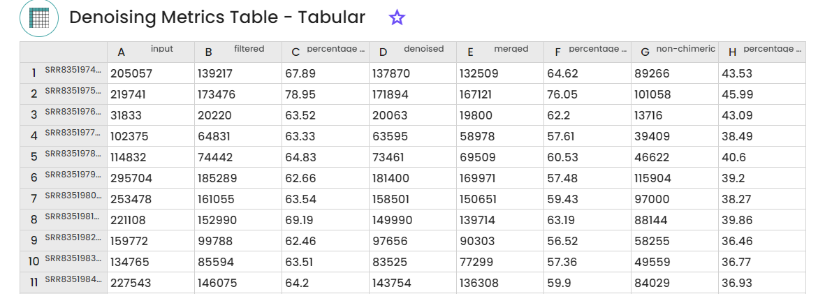
STEP 2 - Denoising, clustering sequences
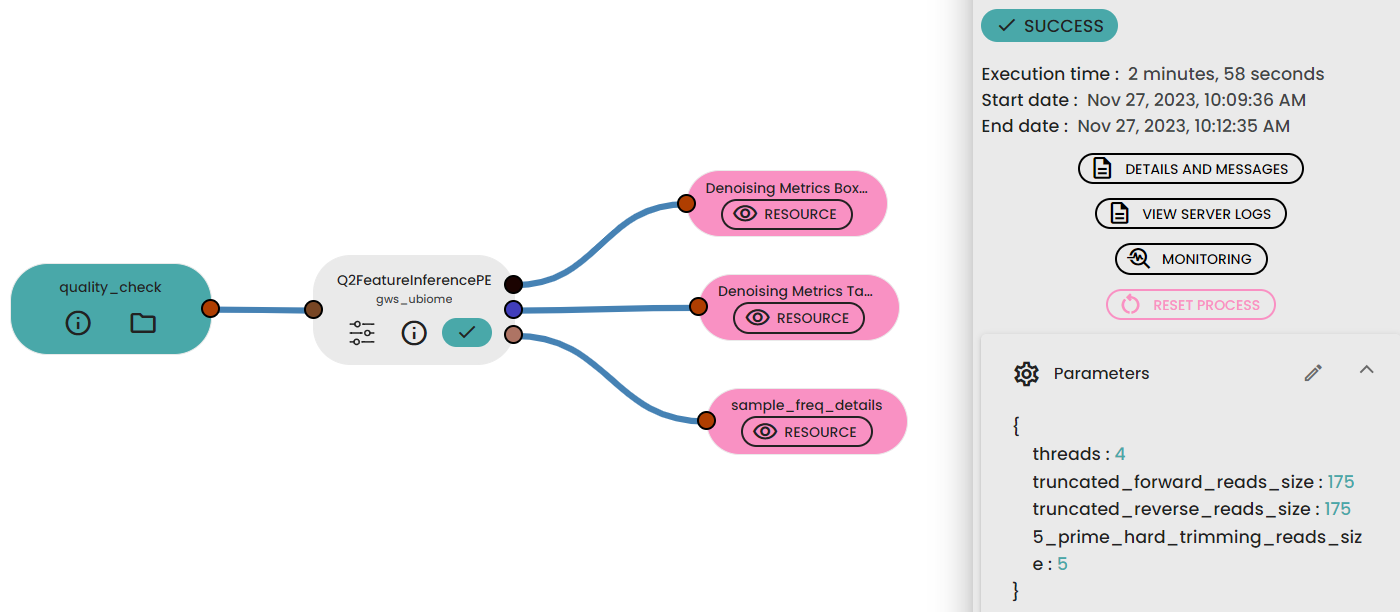
This step method (task: uBiome -Qiime2 featureInference) requires two (paired-end, one for single-end) parameters to trimand filter sequences before joining paired reads to infer ASVs with DADA2.
Files :
Outputs : Feature frequencies folder
Informations :
STEP 3 - Assessing α rarefaction
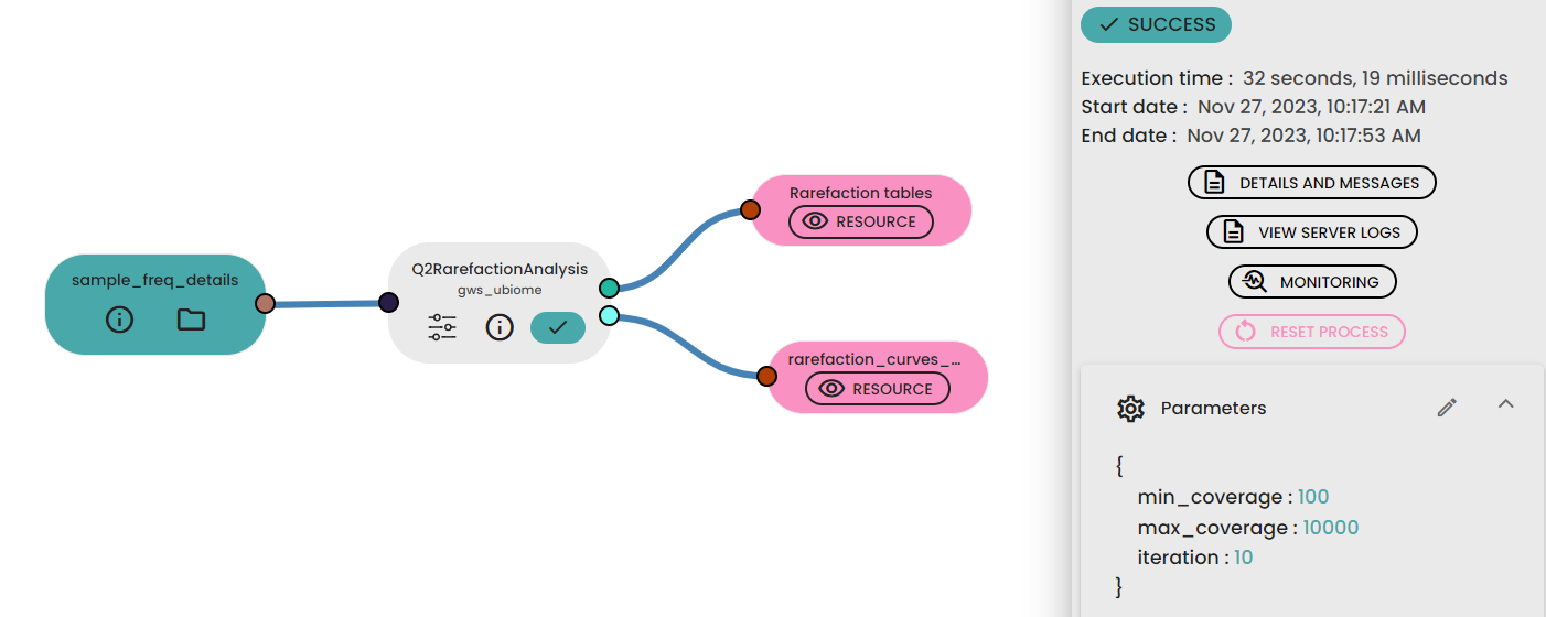
For this step, the max_depth parameter used in the task (uBiome - Qiime2 rarefaction) should be defined by examining the “Frequency per sample” values reported in the Feature table generated previously. In general, a value close to the median of the sample frequencies is recommended, as this usually provides an effective balance between retaining a sufficient sequencing depth and avoiding excessive sample loss. This value can be increased if the rarefaction curves do not yet reach a plateau, or decreased if a substantial number of samples are discarded because of insufficient sequencing depth.
The min_depth parameter was set to 1000 reads; this value was selected empirically as a low starting point for exploring the early part of the rarefaction curves
Files :
Informations :
STEP 4 - Taxonomy, diversity assessments
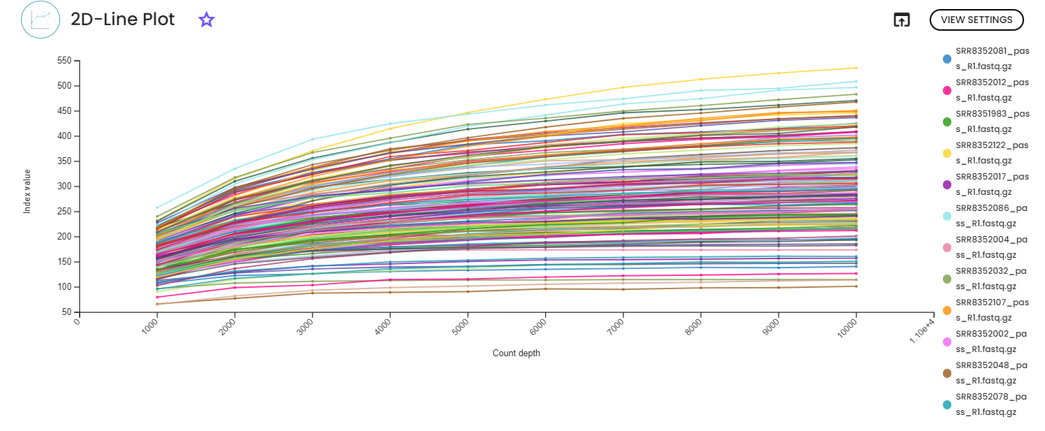
An important parameter that needs to be provided to this step task (task: uBiome - Qiime2 Taxonomy Diversity) is sampling depth, which is the even sampling (i.e., rarefaction) depth. Because most diversity metrics are sensitive to different sampling depths across different samples, this script will randomly subsample the counts from each sample to the value provided for this parameter. For example, if you provide --p-sampling-depth 500, this step will subsample the counts in each sample without replacement so that each sample in the resulting table has a total count of 500. If the total count for any sample(s) are smaller than this value, those samples will be dropped from the diversity analysis.
We recommend making your choice by reviewing the previous rarefication views. Choose a value that is as high as possible (so you retain more sequences per sample) while excluding as few samples as possible. To do so, the visualization file from the previous step will display two lineplots. The plots will display the alpha diversity (observed features or shannon) as a function of the sampling depth. This is used to determine whether the richness or evenness has saturated based on the sampling depth. The rarefaction curve (select the lineplot 2D view) should “level out” as you approach the maximum sampling depth. This plateau value must be evaluated visually.
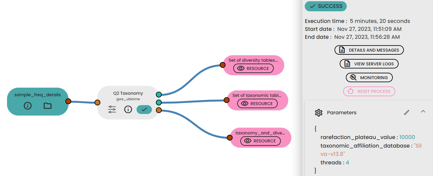
Files :
Outputs : Diversity folder, diversities index table, distance matrix table (PCoA compatible)
Informations :
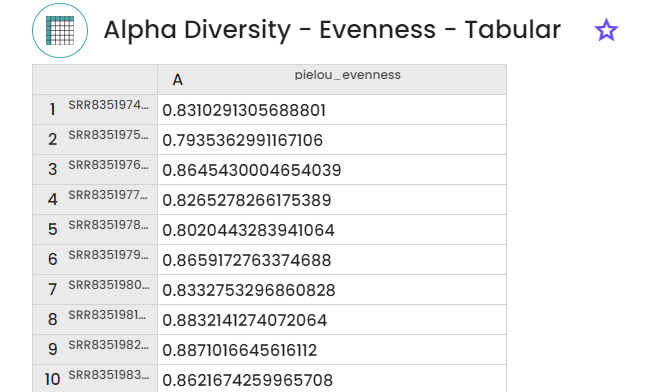
1 - Diversity indexes
- Evenness (
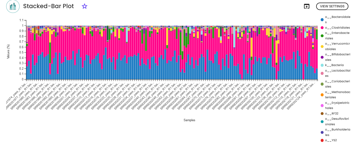
2 - Taxonomic classification
For the classification, we are using a pre-trained Machine-learning-based scikit-learn classifiers, that learn which features best distinguish each taxonomic group, adding an additional step to the classification process. In our case, we are using a Naive Bayes classifier pre-trained on the database Greengenes 13_8 99% OTUs full-length sequences and NCBI-16s full-lenght sequences (from
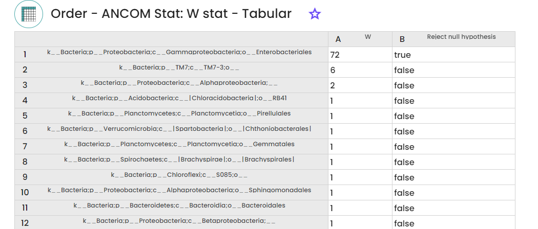
STEP 5 - Samples differential analysis
To use this task
(Task: uBiome - Qiime2 ANCOM differential analysis), , you need to specify the feature table (taxonomic abundance data) and sample metadata with grouping variables to perform the statistical comparison of microbial composition between different sample groups.
This will allow you to assess which taxa have significantly different abundances among your samples.
Files :
Outputs : ANCOM STAT table, Percentile abundances and ANCOM volcano plot table
Informations :
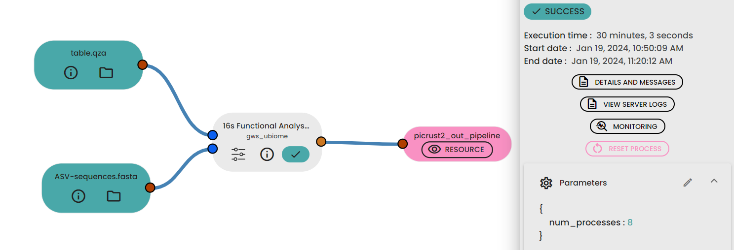
STEP 6 - Functional analysis prediction
This task (uBiome - 16s Functional Analysis Prediction) permit to predict functional analysis of 16s rRNA data . It uses PICRUSt2 : Phylogenetic Investigation of Communities by Reconstruction of Unobserved States.It wraps a number of tools to generate functional predictions based on 16S rRNA gene sequencing data.
Files :
Informations :
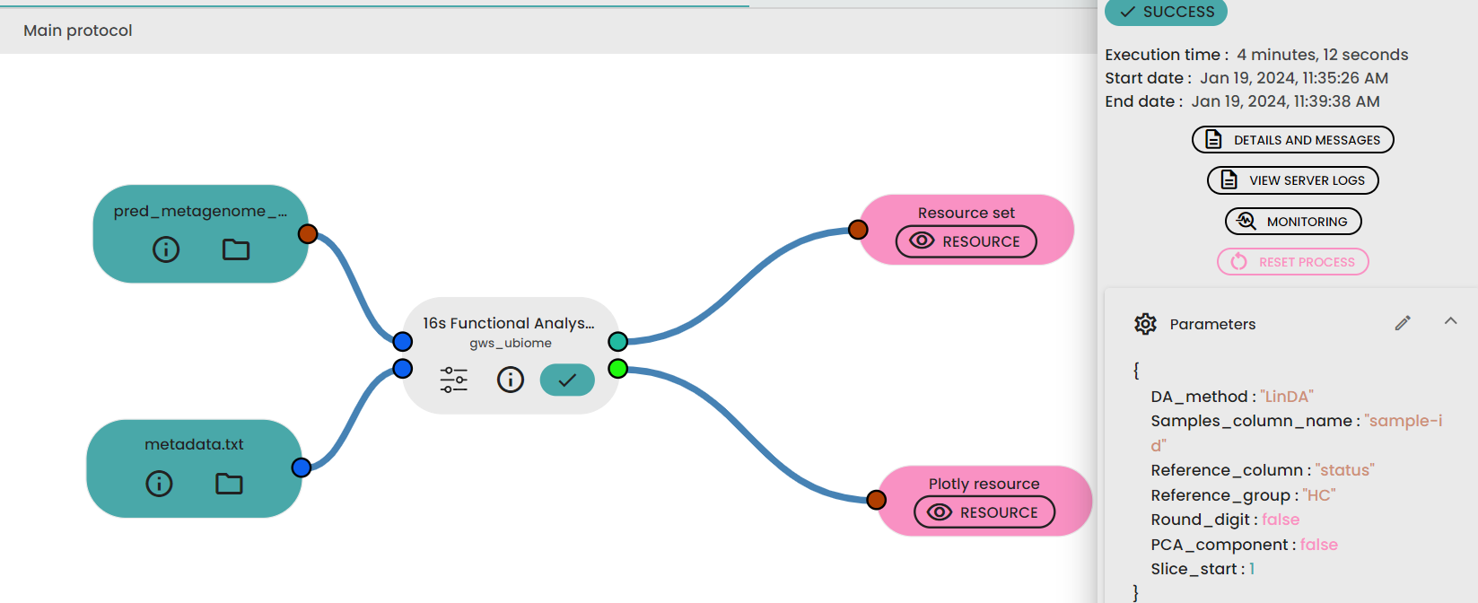
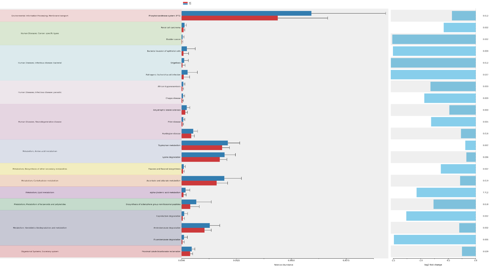
STEP 7 - Functional analysis prediction visualization
This task (uBiome - 16s Functional Analysis Prediction Visualization)permit to analyze and interpret the results of PICRUSt2 functional prediction of 16s rRNA data using ggpicrust2.
Files :
Informations :
