Introduction

We present here a use case on the analysis of the Iris dataset using Principal Component Analysis (PCA) method, using Gaia brick of our platform Constellab. The Iris dataset consists of 50 samples from each of three species of Iris flower (Iris setosa, Iris virginica and Iris versicolor). Four features were measured from each sample: the length and the width of the sepals and petals, in centimeters. Principal Component Analysis (PCA) is a widely used algorithm which aims at identifying the combination of features (principal components, or directions in the feature space) that account for the most variance in the data.

Protocol steps

STEP 1 Data preparation and preview

We start by loading the iris dataset from our computer in the databox of the lab. One can have a preview of the raw dataset by clicking on the imported file.

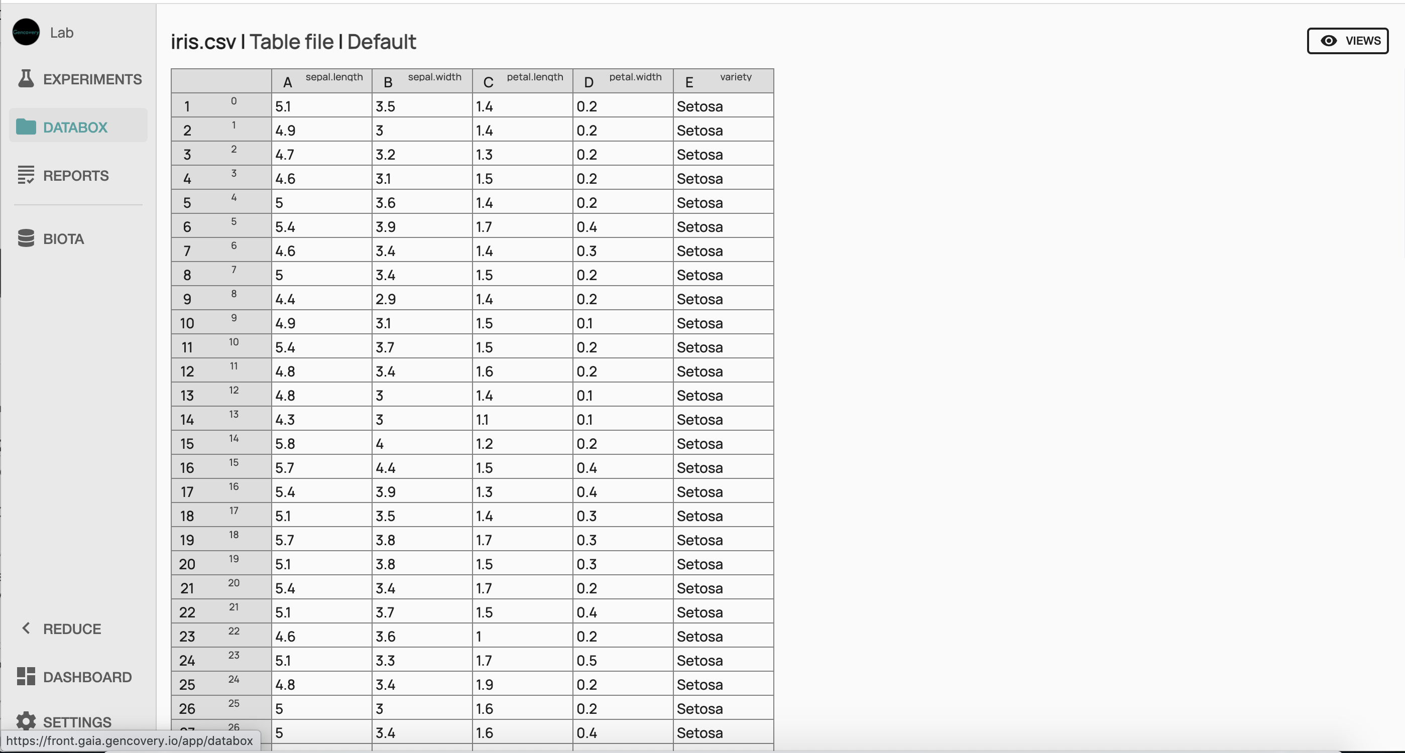
Here the first 4 columns correspond to each of the 4 features of the dataset (the sepal length, the sepal width, the petal length, the petal width, in centimeters), while each line corresponds to a sample of the dataset. The last column indicates the corresponding species (setosa, virginica or versicolor).

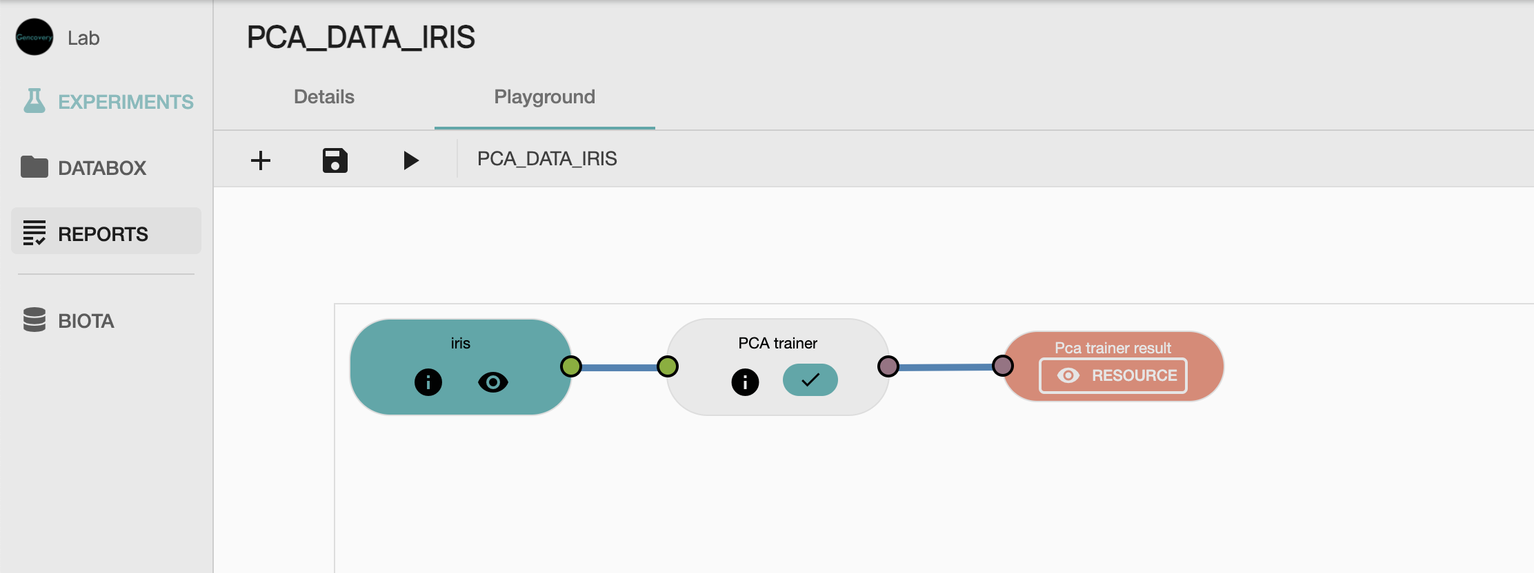
STEP 2 Building of the workflow for the PCA analysis

We start by creating a new experiment which will perform the PCA analysis of the Iris dataset. We then construct the workflow that will be used for our analysis, by selecting :

• the PCA process from our GAIA library,
• the resource containing our processed data as input data, and
• the output process which will collect the result of our analysis.

Some parameters of our processes then need to be specified:

• the parameter of the PCA trainer process determining the number of principal components we want to compute, set here to 2.

STEP 3 Running the PCA workflow analysis and viewing the results

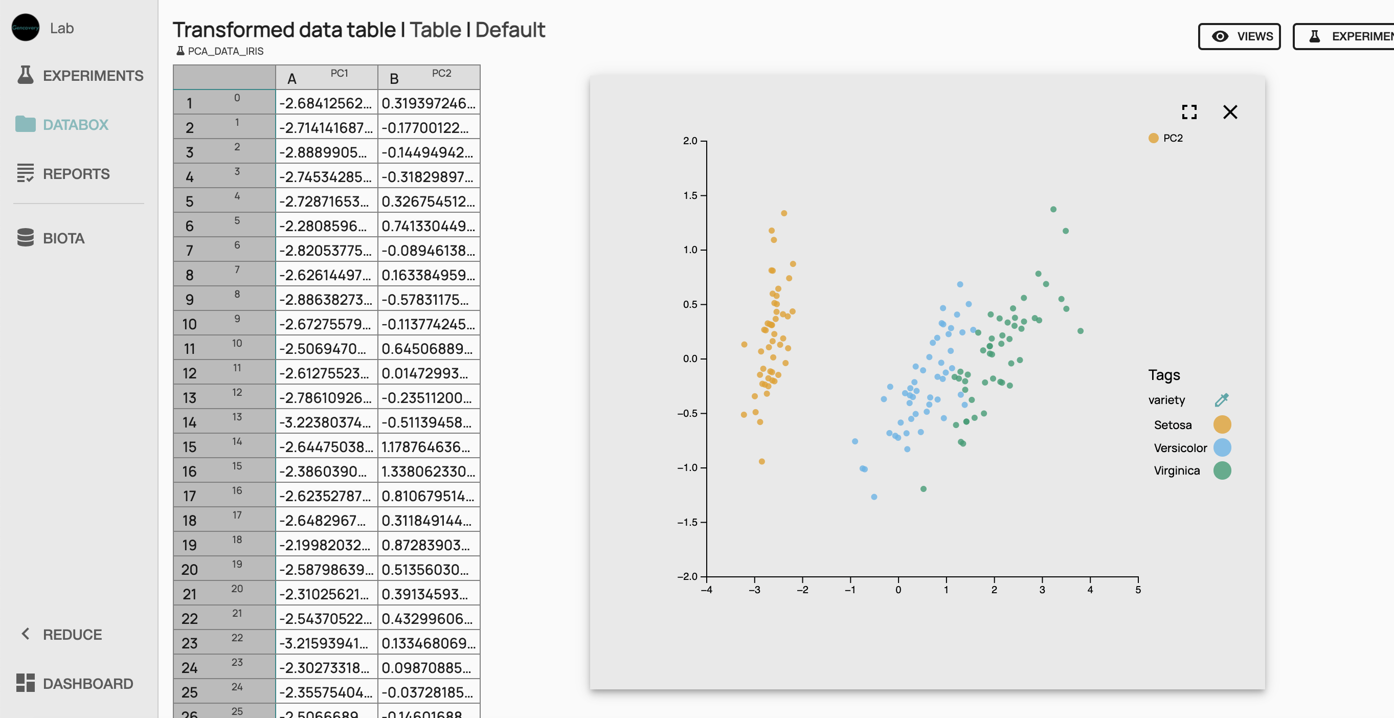
We can now run the experiment which will perform the PCA Analysis of the Iris dataset. Once the experiment has been successfully run, we can access the results in a tabular form, as well as in 2D scatter plot to see the first 2 principal components of the Iris dataset. Each dot of the scatter plot corresponds to a sample of the Iris dataset, while each color denotes the species of the sample. Here, we see a clear separation between setosa species and the other species, whereas versicor et virginica species are less well separated.

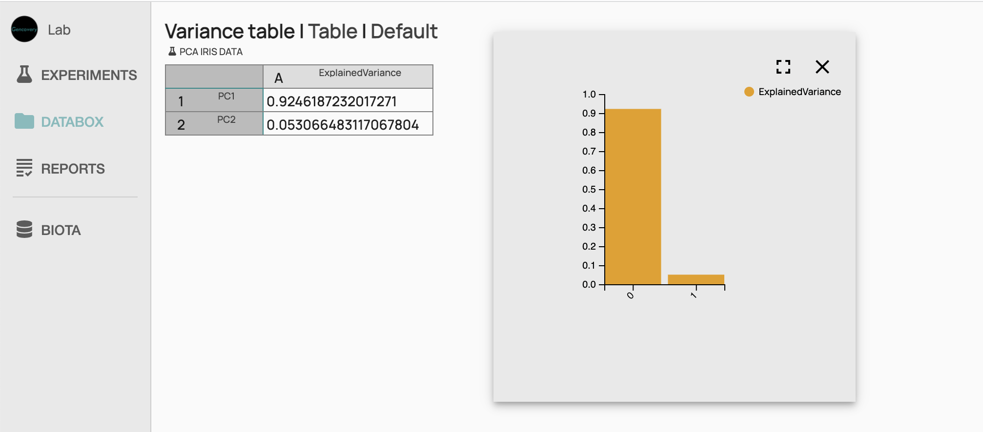
We can further get the variances explained by each component in a bar plot view. Looking at this result, we see that most of the variance of the Iris dataset is explained by the first principal component (more than 90%), while the amount explained by the second component is residual.

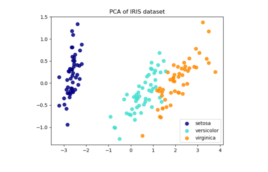
Note that the obtained results on the principal components are similar to the same type of analysis performed in the corresponding example treated in scikit-learn (Learn More).

Once validated, your experiment and your report can be shared among your collaborators.